 The ideal op-amp
has
The ideal op-amp
has
| Objectives: To introduce the basics of digital-to-analog and analog-to-digital conversion and the sampling theorem. |
Topics covered:
Before moving on to digital-to-analog converters (DAC) and analog-to-digital converters (ADC), let us examine some useful fundamentals of analog amplifiers. In particular, you will observe how the op-amp is used to create a DAC and an analog comparator.
With the advent of integrated circuits, the designer of electronic circuits need not be concerned with the inner workings of an IC package, whether digital or analog. Each circuit can be treated as a "black box" and quite often one considers the "ideal" case and ignores the limitations. This is true for analog amplifiers which are also known as operational amplifiers or op-amps for short.
The ideal op-amp
has
These properties mean that the op-amp
That's quite a tall order and real op-amps come very close to the ideal. Observe that you cannot generate an infinite voltage. There is no such thing as a "free lunch". The voltage output from the op-amp will be limited to the supply voltages (called the supply rail). Similarly, the current output will be restricted by the output impedances of the op-amp and the power supply.
Here are typical specifications for the popular "741" operational amplifier.
µA741 op-amp Data Sheet 11 pages, 162KB pdf
|
Ideal op-amp |
741 op-amp |
|
| Voltage Gain |
infinite |
200,000 |
| Bandwidth |
infinite |
1MHz |
| Input Impedance |
infinite |
2M ohms |
| Output Impedance |
0 |
75 ohms |
What this means is that quite often we can design an analog circuit using idealized circuits and not worry about the limitations of the op-amp. The circuits below are some basic ways of using op-amps.
| The slew rate is another measure of the bandwidth of an amplifier. It is a measure of how quickly the output can change and is recorded in units of voltage/time (usually V/µs). |
We think of positive feed-back as having pleasant connotations. In control systems, positive feed-back causes unfettered growth, run-away behaviour and sometimes oscillations. In electronics, negative feed-back is a desirable thing. With lots of excess gain, the op-amp can use negative feed-back to limit the overall voltage gain of the circuit. With negative feed-back come many benefits such as reduced non-linearity and lower output impedance. Negative feed-back is the control mechanism to keep things in check.
 This is the
basic circuit from which all others can be derived. All op-amps are designed to amplify the voltage difference
between the non-inverting (+) and inverting (-) inputs while ignoring any common-mode
signal that may be common to both. The ability to reject the common signal while amplifying the differential input
is called the common-mode rejection ratio (CMRR).
This is the
basic circuit from which all others can be derived. All op-amps are designed to amplify the voltage difference
between the non-inverting (+) and inverting (-) inputs while ignoring any common-mode
signal that may be common to both. The ability to reject the common signal while amplifying the differential input
is called the common-mode rejection ratio (CMRR).
Lots of negative feed-back is used to control the voltage gain of the amplifier.
 Recall the simple
DAC circuit in Chapter 7, Problem 8. By adding an op-amp to
the circuit any loading effect on the resistor network is virtually eliminated.
Recall the simple
DAC circuit in Chapter 7, Problem 8. By adding an op-amp to
the circuit any loading effect on the resistor network is virtually eliminated.
 An analog or voltage
comparator compares two input voltages and determines which is higher or lower. Since the voltage gain is infinite
the output voltage could have only one of two values, equal to the negative or positive supply rail. Thus an input
signal with a continuous analog range is converted to a digital signal. This is a 1-bit ADC.
An analog or voltage
comparator compares two input voltages and determines which is higher or lower. Since the voltage gain is infinite
the output voltage could have only one of two values, equal to the negative or positive supply rail. Thus an input
signal with a continuous analog range is converted to a digital signal. This is a 1-bit ADC.
| What is the output of the comparator when the input voltage Vin is equal to the reference voltage Vref? |
When an analog waveform is sampled, the voltage signal which is continuous in both amplitude and time is digitized. This digitization process results in quantization effects in both domains which lead to important consequences. In the amplitude domain, the resolution is determined by the number of bits of the ADC. Thus an 8-bit ADC can digitize the input signal into 255 voltage steps, equivalent to a precision of 0.4%. The following table shows the effects of various number of ADC bits.
|
No. of ADC bits |
No. of Steps |
Precision |
|
8 |
255 |
0.4 % |
|
10 |
1023 |
0.01 % |
|
12 |
4095 |
0.02 % |
|
14 |
16383 |
0.006 % |
|
16 |
65535 |
0.0015 % |
The resolution in the time domain is determined by the sampling rate, that is, how many samples per second are recorded. The sampling or Nyquist theorem states that the sampling frequency must be at least twice the highest frequency being recorded. The corollary to this is that there must be no frequency component in the signal that is greater than one-half of the sampling frequency.
The sampling theorem can be illustrated graphically. The following diagrams show a sine-wave signal being sampled at different sampling rates. The dashed line represents an approximation of the reconstructed waveform for illustrative purposes.
 Here the sampling
frequency, fs, is the same as the input sine-wave. The reconstructed waveform is a DC value.
Here the sampling
frequency, fs, is the same as the input sine-wave. The reconstructed waveform is a DC value.
 When fs
is increased, the reconstructed waveform is a low frequency signal which is an alias of the true input frequency.
When fs
is increased, the reconstructed waveform is a low frequency signal which is an alias of the true input frequency.
 When fs
is greater than twice the input frequency, the reconstructed waveform has a frequency component that represents
the input waveform.
When fs
is greater than twice the input frequency, the reconstructed waveform has a frequency component that represents
the input waveform.
The Nyquist limit is the highest frequency component which can be recorded for a given sampling frequency. This limit is equal to one-half of the sampling frequency. For example, it is generally accepted that the range of human hearing (and high-fidelity musical recordings) is 20Hz to 20KHz. The standard sampling frequency for digital recordings (CD) is 44.1KHz. It is interesting to note that increasing the sampling frequency does not improve on the quality of the recorded signal. Only the Nyquist limit is raised to a higher level.
A time-varying signal can be represented graphically in a voltage vs time display in the time domain. The same information can be transformed into amplitude vs frequency in the frequency domain. This conversion from the time domain to the frequency domain is performed by the process called Fourier transformation. It is useful to consider the sampling theorem in frequency space.
If the sampling frequency is fs, then the Nyquist limit is fN = ½ fs.
The input frequency fi must be less than the Nyquist limit fN.
More importantly, the corollary of the Nyquist theorem is that there must be no frequency component in the input
signal which is greater than the Nyquist limit.
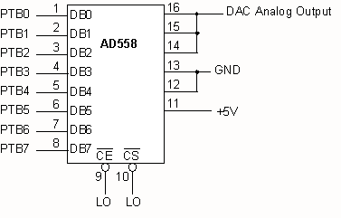 (a) Interface the
AD558 8-bit DAC to a parallel port as shown. Write a simple program to exercise
the DAC as follows. Generate a saw-tooth ramp by outputting the values from
0 to 255 in a continuous loop. Determine the period and frequency of the output
waveform. What information does this reveal about the execution time of your
program?
(a) Interface the
AD558 8-bit DAC to a parallel port as shown. Write a simple program to exercise
the DAC as follows. Generate a saw-tooth ramp by outputting the values from
0 to 255 in a continuous loop. Determine the period and frequency of the output
waveform. What information does this reveal about the execution time of your
program?
(b) Generate a sine wave and display the waveform on the oscilloscope.
AD558 Data Sheet 8 pages, 335KB pdf
 The
tracking ADC is the simplest ADC you can build by adding an up/down counter
and an analog comparator as shown in the block diagram. In this ADC, an incremental
step is made at every clock period in an attempt to get closer to the unknown
input signal. The direction of the desired step is determined by comparing the
output of the DAC with the input signal.
The
tracking ADC is the simplest ADC you can build by adding an up/down counter
and an analog comparator as shown in the block diagram. In this ADC, an incremental
step is made at every clock period in an attempt to get closer to the unknown
input signal. The direction of the desired step is determined by comparing the
output of the DAC with the input signal.
 Construct
the LM311 comparator circuit as shown and interface the output to an input pin
of the MCU. This signal is to be interrogated by the computer in order to determine
the direction of the required step.
Construct
the LM311 comparator circuit as shown and interface the output to an input pin
of the MCU. This signal is to be interrogated by the computer in order to determine
the direction of the required step.
As an alternative, use the internal analog comparator of the MCU.
What is the sampling frequency of your ADC? What is the Nyquist limit?
| The successive approximation algorithm is a classic example of any computer algorithm which may be simple or intricate. In either case, you should always present the solution at first in the form of a flowchart and/or pseudo-code before attempting to write programming instructions. The algorithm must be a complete solution, meaning that if it does not work on paper then you cannot expect its implementation to work. Furthermore, the algorithm must be written in plain language or using algebraic nomenclature. In other words, the solution must be devoid of computer jargon or terminology and must be independent of any computer language or processor architecture. |
Use the internal ADC of the MCU and test using a simple program. Use the internal
timer to record samples every 500µs. Digitize an external sine-wave input
and generate the reconstructed waveform using the AD558 DAC. Compare the input
wave with the reconstructed wave on the oscilloscope. Playback the reconstructed
wave through an audio amplifier and loud-speaker. You may need a low-pass filter
to remove clock frequencies.
2007.01.04